如果这篇文章对你有帮助,欢迎点赞与收藏~
线性规划介绍
线性规划(Linear Programming,LP)是一种在数学规划领域中应用广泛的最优化问题解决方法。其基本思想是在一系列约束条件下,通过建立线性数学模型来描述目标函数,以求得使目标函数最大或最小的决策变量值。线性规划在运筹学、经济学、管理学等领域得到了广泛的应用,能够有效地优化资源分配和决策制定。
线性规划模型
一般线性规划模型可以表示为如下形式:
max ( w ) = c 1 x 1 + c 2 x 2 + … + c n x n s.t. { a 11 x 1 + a 12 x 2 + … + a 1 n x n ≤ b 1 a 21 x 1 + a 22 x 2 + … + a 2 n x n ≤ b 2 … a m 1 x 1 + a m 2 x 2 + … + a m n x n ≤ b m x 1 , x 2 , … , x n ≥ 0 \begin{equation} \begin{aligned} \max(w) = & c_1x_1 + c_2x_2 + \ldots + c_nx_n \\ \text{s.t.} \quad & \left\{ \begin{array}{l} a_{11}x_1 + a_{12}x_2 + \ldots + a_{1n}x_n \leq b_1 \\ a_{21}x_1 + a_{22}x_2 + \ldots + a_{2n}x_n \leq b_2 \\ \ldots \\ a_{m1}x_1 + a_{m2}x_2 + \ldots + a_{mn}x_n \leq b_m \\ \end{array} \right. \\ & x_1, x_2, \ldots, x_n \geq 0 \end{aligned} \end{equation} max(w)=s.t.c1x1+c2x2+…+cnxn⎩ ⎨ ⎧a11x1+a12x2+…+a1nxn≤b1a21x1+a22x2+…+a2nxn≤b2…am1x1+am2x2+…+amnxn≤bmx1,x2,…,xn≥0
其中, w w w为目标函数的值, c 1 , c 2 , … , c n c_1, c_2, \ldots, c_n c1,c2,…,cn为目标函数的系数, x 1 , x 2 , … , x n x_1, x_2, \ldots, x_n x1,x2,…,xn为决策变量, a i j a_{ij} aij为约束条件的系数, b i b_i bi为约束条件的右侧常数。
线性规划的解法
单纯形法
单纯形法是解线性规划问题最经典的方法之一。它通过在可行解空间内移动顶点,逐步逼近最优解。单纯形法的优势在于对于一般情况下能够高效找到最优解,但在特殊情况下可能存在退化、循环等问题。
内点法
内点法是另一种解线性规划问题的方法,它通过在可行解空间内寻找内点,逐步逼近最优解。相比于单纯形法,内点法在处理大规模问题时通常更具优势。
求解工具
在实际应用中,线性规划问题的求解可以借助各种数学建模与求解工具。其中,MATLAB等数学软件提供了强大的线性规划求解功能,使用户能够方便地建立模型、求解问题,并分析优化结果。
线性规划的应用领域
线性规划在实际应用中有着广泛的应用,包括但不限于:
生产计划与资源分配: 在制造业中,线性规划可以用于优化生产计划,确保资源的有效利用,最大程度地提高生产效益。
供应链管理: 在供应链中,线性规划可以帮助优化物流、库存和生产计划,降低成本,提高整体供应链效率。
金融投资组合: 在金融领域,线性规划被用于构建最优的投资组合,以最大化投资回报或降低投资风险。
运输与物流规划: 在交通运输领域,线性规划可用于优化货物运输路线、运输成本,提高物流效率。
市场营销决策: 在市场营销中,线性规划可以用于制定广告投放策略、产品定价策略等,以最大化市场份额或利润。
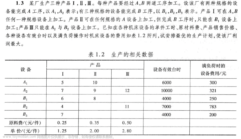
习题1.3
1. 题目要求
2.解题过程
解:
设 使用设备A1生产产品1:x1件,使用设备A2生产产品1:x2件,使用设备B1生产产品1:x3件,使用设备B2生产产品1:x4件,使用设备B3生产产品1:x5件,使用设备A1生产产品2:x6件,使用设备A2生产产品2:x7件,使用设备B1生产产品2:x8件,使用设备A1(B1)生产产品3:x9件。
梳理如下:
- 产品1:设备A1生产x1件,设备A2生产x2件,设备B1生产x3件,设备B2生产x4件,设备B3生产x5件
- 产品2:设备A1生产x6件,设备A2生产x7件,设备B1生产x8件
- 产品3:设备A1和B1共同生产x9件
值得注意的是,上述所有变量都是整数。
由题目所给数据可建立如下线性规划模型:
max w = ( 1.25 − 0.25 ) × ( x 1 + x 2 ) + ( 2 − 0.35 ) × ( x 6 + x 7 ) + ( 2.8 − 0.5 ) × x 9 − 300 6000 × ( 5 x 1 + 10 x 6 ) − 321 10000 × ( 7 x 2 + 9 x 7 + 12 x 9 ) − 250 4000 × ( 6 x 3 + 8 x 8 ) − 783 7000 × ( 4 x 4 + 11 x 9 ) − 200 4000 × 7 x 5 s.t. { 5 x 1 + 10 x 6 ⩽ 6000 7 x 2 + 9 x 7 + 12 x 9 ⩽ 10 6 x 3 + 8 x 8 ⩽ 4000 4 x 4 + 11 x 9 ⩽ 7000 7 x 5 ⩽ 4000 x 1 + x 2 = x 3 + x 4 + x 5 x 6 + x 7 = x 8 x i ⩾ 0 , i = 1 , 2 , ⋯ , 9 \begin{equation} \begin{aligned} \max w = & (1.25-0.25) \times (x_{1}+x_{2}) + (2-0.35) \times (x_{6}+x_{7}) + (2.8-0.5) \times x_{9} \\ & -\frac{300}{6000} \times (5 x_{1}+10 x_{6}) - \frac{321}{10000} \times (7 x_{2}+9 x_{7}+12 x_{9}) \\ & -\frac{250}{4000} \times (6 x_{3}+8 x_{8}) - \frac{783}{7000} \times (4 x_{4}+11 x_{9}) - \frac{200}{4000} \times 7 x_{5} \\ \text{s.t.} \quad & \left\{ \begin{array}{l} 5 x_{1}+10 x_{6} \leqslant 6000 \\ 7 x_{2}+9 x_{7}+12 x_{9} \leqslant 10 \\ 6 x_{3}+8 x_{8} \leqslant 4000 \\ 4 x_{4}+11 x_{9} \leqslant 7000 \\ 7 x_{5} \leqslant 4000 \\ x_{1}+x_{2} = x_{3}+x_{4}+x_{5} \\ x_{6}+x_{7} = x_{8} \\ x_{i} \geqslant 0, \quad i=1,2, \cdots, 9 \end{array} \right. \end{aligned} \end{equation} maxw=s.t.(1.25−0.25)×(x1+x2)+(2−0.35)×(x6+x7)+(2.8−0.5)×x9−6000300×(5x1+10x6)−10000321×(7x2+9x7+12x9)−4000250×(6x3+8x8)−7000783×(4x4+11x9)−4000200×7x5⎩ ⎨ ⎧5x1+10x6⩽60007x2+9x7+12x9⩽106x3+8x8⩽40004x4+11x9⩽70007x5⩽4000x1+x2=x3+x4+x5x6+x7=x8xi⩾0,i=1,2,⋯,9
化成MATLAB标准型,即:
min w = ( − 1 ) ∗ [ ( 1.25 − 0.25 ) × ( x 1 + x 2 ) + ( 2 − 0.35 ) × ( x 6 + x 7 ) + ( 2.8 − 0.5 ) × x 9 − 300 6000 × ( 5 x 1 + 10 x 6 ) − 321 10000 × ( 7 x 2 + 9 x 7 + 12 x 9 ) − 250 4000 × ( 6 x 3 + 8 x 8 ) − 783 7000 × ( 4 x 4 + 11 x 9 ) − 200 4000 × 7 x 5 ] s. t. { [ 5 0 0 0 0 10 0 0 0 0 7 0 0 0 0 9 0 12 0 0 6 0 0 0 0 8 0 0 0 0 4 0 0 0 0 11 0 0 0 0 7 0 0 0 0 ] [ x 1 x 2 x 3 x 4 x 5 x 6 x 7 x 8 x 9 ] ⩽ [ 6000 10000 4000 7000 4000 ] [ 1 1 − 1 − 1 − 1 0 0 0 0 0 0 0 0 0 1 1 − 1 0 ] [ x 1 x 2 x 3 x 4 x 5 x 6 x 7 x 8 x 9 ] = [ 0 0 ] x i ⩾ 0 , i = 1 , 2 , ⋯ , 9 \begin{equation} \begin{aligned} \min w=(-1)*[(1.25-0.25)\times\left(x_{1}+x_{2}\right)+(2-0.35)\times\left(x_{6}+x_{7}\right)+(2.8-0.5)\times x_{9} \\ -\frac{300}{6000}\times\left(5 x_{1}+10 x_{6}\right)-\frac{321}{10000}\times\left(7 x_{2}+9 x_{7}+12 x_{9}\right) \\ -\frac{250}{4000}\times\left(6 x_{3}+8 x_{8}\right)-\frac{783}{7000}\times\left(4 x_{4}+11 x_{9}\right)-\frac{200}{4000} \times 7 x_{5}] \\ \text { s. t. }\left\{ \begin{array}{l} \begin{bmatrix} 5 & 0 & 0 & 0 & 0 & 10 & 0 & 0 & 0\\ 0 & 7 & 0 & 0 & 0 & 0 & 9 & 0 & 12\\ 0 & 0 & 6 & 0 & 0 & 0 & 0 & 8 & 0\\ 0 & 0 & 0 & 4 & 0 & 0 & 0 & 0 & 11\\ 0 & 0 & 0 & 0 & 7 & 0 & 0 & 0 & 0\\ \end{bmatrix} \begin{bmatrix} x_1 \\ x_2 \\ x_3 \\ x_4 \\ x_5 \\ x_6 \\ x_7 \\ x_8 \\ x_9 \\ \end{bmatrix} \leqslant \begin{bmatrix} 6000 \\ 10000 \\ 4000 \\ 7000 \\ 4000 \end{bmatrix} \\ \begin{bmatrix} 1 & 1 & -1 & -1 & -1 & 0 & 0 & 0 & 0 \\ 0 & 0 & 0 & 0 & 0 & 1 & 1 & -1 & 0 \end{bmatrix} \begin{bmatrix} x_1 \\ x_2 \\ x_3 \\ x_4 \\ x_5 \\ x_6 \\ x_7 \\ x_8 \\ x_9 \\ \end{bmatrix} = \begin{bmatrix} 0 \\ 0 \end{bmatrix} \\ x_{i} \geqslant 0, i=1,2, \cdots, 9 \end{array}\right. \end{aligned} \end{equation} minw=(−1)∗[(1.25−0.25)×(x1+x2)+(2−0.35)×(x6+x7)+(2.8−0.5)×x9−6000300×(5x1+10x6)−10000321×(7x2+9x7+12x9)−4000250×(6x3+8x8)−7000783×(4x4+11x9)−4000200×7x5] s. t. ⎩ ⎨ ⎧ 500000700000600000400000710000009000008000120110 x1x2x3x4x5x6x7x8x9 ⩽ 600010000400070004000 [1010−10−10−1001010−100] x1x2x3x4x5x6x7x8x9 =[00]xi⩾0,i=1,2,⋯,9
3.程序
求解的MATLAB程序如下:
clc , clear

% pr:profit 每个产品的净利润
pr1 = 1.25 - 0.25;
pr2 = 2 - 0.35;
pr3 = 2.8 - 0.5;

pr = [pr1 * ones(1, 2), zeros(1, 3), pr2 * ones(1, 2), 0, pr3]; % 利润矩阵

% ec:equipment cost 每个设备的单位运行费用
ec1 = 300 / 6000;
ec2 = 321 / 10000;
ec3 = 250 / 4000;
ec4 = 783 / 7000;
ec5 = 200 / 4000;

ec = [5 * ec1, 7 * ec2, 6 * ec3, 4 * ec4, 7 * ec5, 10 * ec1, 9 * ec2, 8 * ec3, 12 * ec2 + 11 * ec4]; % 设备费用矩阵
% 易错:注意这里要乘以运行时长!

f = pr - ec; % 计算出销售利润与机器成本的和矩阵,也就是最终收益
f = -f; % 求min

A = [5, 0, 0, 0, 0, 10, 0, 0, 0; ...
    0, 7, 0, 0, 0, 0, 9, 0, 12; ...
    0, 0, 6, 0, 0, 0, 0, 8, 0; ...
    0, 0, 0, 4, 0, 0, 0, 0, 11; ...
    0, 0, 0, 0, 7, 0, 0, 0, 0];
b = [6000, 10000, 4000, 7000, 4000];

Aeq = [1, 1, -1, -1, -1, 0, 0, 0, 0; ...
    0, 0, 0, 0, 0, 1, 1, -1, 0];
beq = zeros(2, 1);

intcon = 1:9;
[x, w] = intlinprog(f, intcon, A, b, Aeq, beq, zeros(9, 1));
w = -w; % 求max

% 输出结果
format shortG;
x
w
4.结果
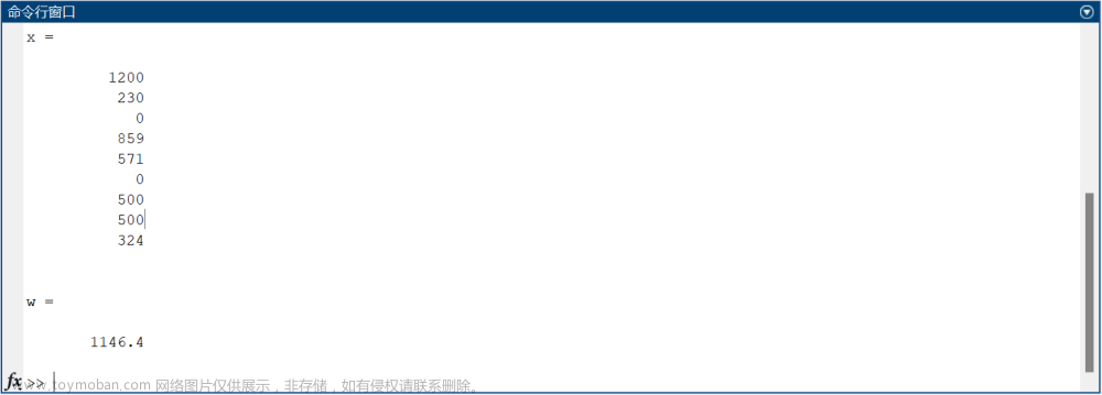
求得的最优解是:
使用设备A1生产产品1:1200件,使用设备A2生产产品1:230件,使用设备B1生产产品1:0件,使用设备B2生产产品1:859件,使用设备B3生产产品1:571件,使用设备A1生产产品2:0件,使用设备A2生产产品2:500件,使用设备B1生产产品2:500件,使用设备A1和B1生产产品3:324件。
最大利润:1146.4(元)
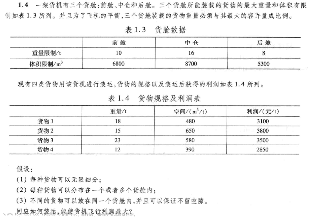
习题1.4
1.题目要求
2.解题过程
解:
设 前舱装运货物1:x1吨,前舱装运货物2:x2吨,前舱装运货物3:x3吨,前舱装运货物4:x4吨
中舱装运货物1:x5吨,中舱装运货物2:x6吨,中舱装运货物3:x7吨,中舱装运货物4:x8吨
后舱装运货物1:x9吨,后舱装运货物2:x10吨,后舱装运货物3:x11吨,后舱装运货物4:x12吨
由题目所给数据可建立如下线性规划模型:
max
w
=
3100
×
(
x
1
+
x
5
+
x
9
)
+
3800
×
(
x
2
+
x
6
+
x
10
)
+
3500
×
(
x
3
+
x
7
+
x
11
)
+
2850
×
(
x
4
+
x
8
+
x
12
)
s. t.
{
x
1
+
x
5
+
x
9
⩽
18
x
2
+
x
6
+
x
10
⩽
15
x
3
+
x
7
+
x
11
⩽
23
x
4
+
x
8
+
x
12
⩽
10
x
1
+
x
2
+
x
3
+
x
4
⩽
10
x
5
+
x
6
+
x
7
+
x
8
⩽
16
x
9
+
x
10
+
x
11
+
x
12
⩽
8
480
x
1
+
650
x
2
+
580
x
3
+
390
x
4
⩽
6800
480
x
5
+
650
x
6
+
580
x
7
+
390
x
8
⩽
8700
480
x
9
+
650
x
10
+
580
x
11
+
390
x
12
⩽
5300
16
(
x
1
+
x
2
+
x
3
+
x
4
)
=
10
(
x
5
+
x
6
+
x
7
+
x
8
)
8
(
x
5
+
x
6
+
x
7
+
x
8
)
=
16
(
x
9
+
x
10
+
x
11
+
x
12
)
x
i
⩾
0
,
i
=
1
,
2
,
⋯
,
12
\begin{equation} \begin{aligned} \max w=3100\times\left(x_{1}+x_{5}+x_{9}\right)+3800\times\left(x_{2}+x_{6}+x_{10}\right)+3500\times \left(x_{3}+x_{7}+x_{11}\right)+2850\times\left(x_{4}+x_{8}+x_{12}\right) \\ \text { s. t. }\left\{ \begin{array}{l} x_{1}+ x_{5}+x_{9} \leqslant 18 \\ x_{2}+ x_{6}+x_{10} \leqslant 15 \\ x_{3}+ x_{7}+x_{11} \leqslant 23 \\ x_{4}+ x_{8}+x_{12} \leqslant 10 \\ x_{1}+ x_{2}+x_{3}+ x_{4} \leqslant 10 \\ x_{5}+ x_{6}+x_{7}+ x_{8} \leqslant 16 \\ x_{9}+ x_{10}+x_{11}+ x_{12} \leqslant 8 \\ 480x_{1}+ 650x_{2}+580x_{3}+ 390x_{4} \leqslant 6800 \\ 480x_{5}+ 650x_{6}+580x_{7}+ 390x_{8} \leqslant 8700 \\ 480x_{9}+ 650x_{10}+580x_{11}+ 390x_{12} \leqslant 5300 \\ 16(x_{1}+ x_{2}+x_{3}+ x_{4})=10(x_{5}+ x_{6}+x_{7}+ x_{8})\\ 8(x_{5}+ x_{6}+x_{7}+ x_{8})=16(x_{9}+ x_{10}+x_{11}+ x_{12})\\ x_{i} \geqslant 0, i=1,2, \cdots, 12 \end{array}\right. \\ \end{aligned} \end{equation}
maxw=3100×(x1+x5+x9)+3800×(x2+x6+x10)+3500×(x3+x7+x11)+2850×(x4+x8+x12) s. t. ⎩
⎨
⎧x1+x5+x9⩽18x2+x6+x10⩽15x3+x7+x11⩽23x4+x8+x12⩽10x1+x2+x3+x4⩽10x5+x6+x7+x8⩽16x9+x10+x11+x12⩽8480x1+650x2+580x3+390x4⩽6800480x5+650x6+580x7+390x8⩽8700480x9+650x10+580x11+390x12⩽530016(x1+x2+x3+x4)=10(x5+x6+x7+x8)8(x5+x6+x7+x8)=16(x9+x10+x11+x12)xi⩾0,i=1,2,⋯,12
化成MATLAB标准型,即:
min w = ( − 1 ) ∗ [ 3100 × ( x 1 + x 5 + x 9 ) + 3800 × ( x 2 + x 6 + x 10 ) + 3500 × ( x 3 + x 7 + x 11 ) + 2850 × ( x 4 + x 8 + x 12 ) ] s. t. { [ 1 0 0 0 1 0 0 0 1 0 0 0 0 1 0 0 0 1 0 0 0 1 0 0 0 0 1 0 0 0 1 0 0 0 1 0 0 0 0 1 0 0 0 1 0 0 0 1 1 1 1 1 0 0 0 0 0 0 0 0 0 0 0 0 1 1 1 1 0 0 0 0 0 0 0 0 0 0 0 0 1 1 1 1 480 650 580 390 0 0 0 0 0 0 0 0 0 0 0 0 480 650 580 390 0 0 0 0 0 0 0 0 0 0 0 0 480 650 580 390 ] [ x 1 x 2 x 3 x 4 x 5 x 6 x 7 x 8 x 9 x 10 x 11 x 12 ] ⩽ [ 18 15 23 12 10 16 8 6800 8700 5300 ] [ 8 8 8 8 − 5 − 5 − 5 − 5 0 0 0 0 0 0 0 0 1 1 1 1 − 2 − 2 − 2 − 2 ] [ x 1 x 2 x 3 x 4 x 5 x 6 x 7 x 8 x 9 x 10 x 11 x 12 ] = [ 0 0 ] x i ⩾ 0 , i = 1 , 2 , ⋯ , 12 \begin{equation} \begin{aligned} \min w=(-1)*[3100\times\left(x_{1}+x_{5}+x_{9}\right)+3800\times\left(x_{2}+x_{6}+x_{10}\right)+3500\times \left(x_{3}+x_{7}+x_{11}\right)+2850\times\left(x_{4}+x_{8}+x_{12}\right) ]\\ \text { s. t. }\left\{ \begin{array}{l} \begin{bmatrix} 1 & 0 & 0 & 0 & 1 & 0 & 0 & 0 & 1 & 0 & 0 & 0 \\ 0 & 1 & 0 & 0 & 0 & 1 & 0 & 0 & 0 & 1 & 0 & 0 \\ 0 & 0 & 1 & 0 & 0 & 0 & 1 & 0 & 0 & 0 & 1 & 0 \\ 0 & 0 & 0 & 1 & 0 & 0 & 0 & 1 & 0 & 0 & 0 & 1 \\ 1 & 1 & 1 & 1 & 0 & 0 & 0 & 0 & 0 & 0 & 0 & 0 \\ 0 & 0 & 0 & 0 & 1 & 1 & 1 & 1 & 0 & 0 & 0 & 0 \\ 0 & 0 & 0 & 0 & 0 & 0 & 0 & 0 & 1 & 1 & 1 & 1 \\ 480 & 650 & 580 & 390 & 0 & 0 & 0 & 0 & 0 & 0 & 0 & 0 \\ 0 & 0 & 0 & 0 & 480 & 650 & 580 & 390 & 0 & 0 & 0 & 0 \\ 0 & 0 & 0 & 0 & 0 & 0 & 0 & 0 & 480 & 650 & 580 & 390 \end{bmatrix} \begin{bmatrix} x_1 \\ x_2 \\ x_3 \\ x_4 \\ x_5 \\ x_6 \\ x_7 \\ x_8 \\ x_9 \\x_{10} \\ x_{11} \\ x_{12} \end{bmatrix} \leqslant \begin{bmatrix} 18 \\ 15 \\ 23 \\ 12 \\ 10 \\ 16 \\ 8 \\ 6800 \\ 8700 \\ 5300 \end{bmatrix} \\ \begin{bmatrix} 8 & 8 & 8 & 8 & -5 & -5 & -5 & -5 & 0 & 0 & 0 & 0 \\ 0 & 0 & 0 & 0 & 1 & 1 & 1 & 1 & -2 & -2 & -2 & -2 \\ \end{bmatrix} \begin{bmatrix} x_1 \\ x_2 \\ x_3 \\ x_4 \\ x_5 \\ x_6 \\ x_7 \\ x_8 \\ x_9 \\x_{10} \\ x_{11} \\ x_{12} \end{bmatrix} = \begin{bmatrix} 0 \\ 0 \end{bmatrix} \\ x_{i} \geqslant 0, i=1,2, \cdots, 12 \end{array}\right. \\ \end{aligned} \end{equation} minw=(−1)∗[3100×(x1+x5+x9)+3800×(x2+x6+x10)+3500×(x3+x7+x11)+2850×(x4+x8+x12)] s. t. ⎩ ⎨ ⎧ 100010048000010010065000001010058000000110039000100001004800010001006500001001005800000101003900100000100480010000100650001000100580000100100390 x1x2x3x4x5x6x7x8x9x10x11x12 ⩽ 1815231210168680087005300 [80808080−51−51−51−510−20−20−20−2] x1x2x3x4x5x6x7x8x9x10x11x12 =[00]xi⩾0,i=1,2,⋯,12
3.程序
clc , clear

% 按行展开获得f
f = [3100 * ones(3, 1), 3800 * ones(3, 1), 3500 * ones(3, 1), 2850 * ones(3, 1)];
f = f';
f = f(:)';
f = -f; % 求min

A1 = [eye(4), eye(4), eye(4)];
A2 = blkdiag(ones(1, 4), ones(1, 4), ones(1, 4));
A3 = blkdiag([480, 650, 580, 390], [480, 650, 580, 390], [480, 650, 580, 390]);
A = vertcat(A1, A2, A3);

b = [18, 15, 23, 12, 10, 16, 8, 6800, 8700, 5300];

Aeq1 = [8 * ones(1, 4), -5 * ones(1, 4), zeros(1, 4)];
Aeq2 = [zeros(1, 4), ones(1, 4), -2 * ones(1, 4)];
Aeq = vertcat(Aeq1, Aeq2);

beq = zeros(2, 1);

% 获得结果
[x, w] = linprog(f, A, b, Aeq, beq, zeros(12, 1));

format longG;
% 转化为3*4的矩阵
x = reshape(x, [4, 3])'
% 求和
x = sum(x)
% 利润
w = -w % 求max
4.结果
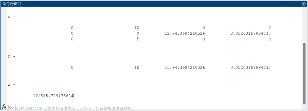
求得的最优解是:
前舱装运货物1:x1 = 0 吨 前舱装运货物2:x2 = 10.0000 吨 前舱装运货物3:x3 = 0 吨 前舱装运货物4:x4 = 0 吨
中舱装运货物1:x5 = 0 吨 中舱装运货物2:x6 = 0 吨 中舱装运货物3:x7 = 12.9474 吨 中舱装运货物4:x8 = 3.0526 吨
后舱装运货物1:x9 = 0 吨 后舱装运货物2:x10 = 5.0000 吨 后舱装运货物3:x11 = 3.0000 吨 后舱装运货物4:x12 = 0 吨
货物1的总装运量:x1 + x5 + x9 = 0 + 0 + 0 = 0 吨
货物2的总装运量:x2 + x6 + x10 = 10.0000 + 0 + 5.0000 = 15.0000 吨
货物3的总装运量:x3 + x7 + x11 = 0 + 12.9474 + 3.0000 = 15.9474 吨
货物4的总装运量:x4 + x8 + x12 = 0 + 3.0526 + 0 = 3.0526 吨
最大利润:121515.789(元)文章来源:https://www.toymoban.com/news/detail-757113.html
如果这篇文章对你有帮助,欢迎点赞与收藏~文章来源地址https://www.toymoban.com/news/detail-757113.html
到了这里,关于【数学建模】《实战数学建模:例题与讲解》第二讲-线性规划(含Matlab代码)的文章就介绍完了。如果您还想了解更多内容,请在右上角搜索TOY模板网以前的文章或继续浏览下面的相关文章,希望大家以后多多支持TOY模板网!